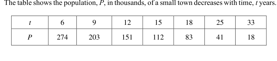
The table shows the population, $P$, in thousands, of a small town decreases with time, $t$ years.

1. Calculate the values of $\ln P$ for each corresponding value of $t$ to 2 decimal places.

For $P = 274$, $\ln P = \ln 274 \approx 5.61$
For $P = 203$, $\ln P = \ln 203 \approx 5.31$
For $P = 151$, $\ln P = \ln 151 \approx 5.02$
For $P = 112$, $\ln P = \ln 112 \approx 4.72$
For $P = 83$, $\ln P = \ln 83 \approx 4.42$
For $P = 41$, $\ln P = \ln 41 \approx 3.71$
For $P = 18$, $\ln P = \ln 18 \approx 2.89$

2. Plot the points $(t, \ln P)$ on the given grid and draw a straight line of best fit.

Plot the coordinates $(6, 5.61)$, $(9, 5.31)$, $(12, 5.02)$, $(15, 4.72)$, $(18, 4.42)$, $(25, 3.71)$, and $(33, 2.89)$ on the grid with $t$ on the horizontal axis and $\ln P$ on the vertical axis. Draw a straight line passing through these points.

1. Calculate the gradient of the straight line graph of $\ln P$ against $t$

Using the points $(6, \ln 274)$ and $(33, \ln 18)$ from the table:
Gradient $m = \frac{\ln 18 - \ln 274}{33 - 6}$
$m = \frac{2.8904 - 5.6131}{27} \approx -0.1008$
Gradient $\approx -0.1$ (to 1 d.p.)

2. Relate the given non-linear equation to the linear form

$P = Ae^{-kt}$
Taking natural logarithms on both sides:
$\ln P = \ln(Ae^{-kt})$
$\ln P = -kt + \ln A$
This is in the form $Y = mX + c$, where $Y = \ln P$, $X = t$, gradient $m = -k$, and vertical intercept $c = \ln A$.

3. Find the value of $k$

Since $m = -k$:
$-k = -0.1008$
$k \approx 0.1$ (to 1 d.p.)

4. Find the value of $A$ and state the final equation

Using the point $(6, 5.6131)$ to find the intercept $c$:
$5.6131 = -0.1008(6) + \ln A$
$\ln A = 5.6131 + 0.6048 = 6.2179$
$A = e^{6.2179} \approx 501.6$
$A = 500$ (to the nearest hundred)
Therefore, $P = 500e^{-0.1t}$.

1. Set up the inequality or equation using the model from part (b)

From part (b), the model is $P = 500e^{-0.1t}$.
Since $P$ is in thousands, a population of $100\,000$ corresponds to $P = 100$.
We require $P < 100$:
$500e^{-0.1t} < 100$

2. Solve for $t$

$e^{-0.1t} < \frac{100}{500}$
$e^{-0.1t} < 0.2$
$-0.1t < \ln 0.2$
$t > \frac{\ln 0.2}{-0.1}$
$t > 16.094$

3. State the final answer to the nearest year

To the nearest year, $t = 16$.