An experiment was conducted with a ramp placed on top of a table. A ball is then released from the ramp, at a height mm above the table. When the ball leaves the ramp's edge, it travels in a parabolic motion to the floor. The horizontal distance travelled by the ball before it lands, mm, is then measured and recorded.
Observations at different heights are captured in the following table:
100 200 300 450 600 800 1000 253 337 395 451 495 534 573
The value of the product moment correlation coefficient, , for this data is 0.962, correct to 3 significant figures.
| 100 | 200 | 300 | 450 | 600 | 800 | 1000 | |
|---|---|---|---|---|---|---|---|
| 253 | 337 | 395 | 451 | 495 | 534 | 573 |
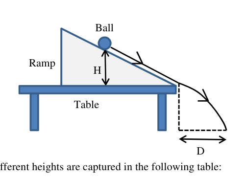
- (i)
Sketch a scatter diagram for the above data.
- (ii)
Using the diagram in (i), explain why it is insufficient to rely on the value of to indicate a linear relationship between any two variables.
- (iii)
It is thought that the horizontal distance can be modelled by
Explain which of the above models would provide a better estimate of for a given value of . - (iv)
Using the model chosen in (iii) and an appropriate regression line, find the value of when mm.
- (v)
Comment on the reliability of the estimate of when mm, as compared to the estimate obtained in (iv).
It won't just hand you the answer — it asks where you're stuck.How the checker works
Worked solution
13(i)
1. Set up axes and sketch the scatter diagram by plotting the points from the table.
Draw a horizontal axis labelled and a vertical axis labelled .
Plot the pairs of to accurately reflect their relative positions, showing a sequence of points that curves downwards (concave down) as increases.
[A sketched graph with the horizontal axis labelled and vertical axis labelled , containing 7 points plotted at their approximate relative positions: , , , , , , and . The points should exhibit a clear increasing trend with a decreasing gradient.]
13(ii)
1. Observe the shape of the data points from the scatter diagram.
The scatter diagram in (i) shows that the data points follow a curvilinear path rather than a straight line, which implies a non-linear relationship between and .
2. Contrast the visual observation with the given $r$ value.
The product moment correlation coefficient is very close to . If one were to rely solely on , one might mistakenly conclude there is a strong positive linear correlation. This proves that a high value can be present even when the actual relationship is non-linear.
From the scatter diagram in (i), the data points lie on a curve, indicating a non-linear relationship between and . However, the calculated value of is , which is close to and might wrongly suggest a strong positive linear relationship. Thus, relying solely on is insufficient to conclude linearity; the scatter diagram must also be visually inspected.
13(iii)
1. Calculate the product moment correlation coefficient ($r$) for both proposed linear models using a graphing calculator
Using a graphing calculator,
For (i.e. against ),
For (i.e. against ),
2. Compare the $r$ values to deduce the better model
Since , the value of for the model is closer to .
Therefore, the data points for and lie closer to a straight line, making the better model.
The model provides a better estimate because its product moment correlation coefficient is closer to .
13(iv)
1. Identify the model from (iii) and state the equation of the appropriate regression line.
From (iii), the linear model is chosen because the product moment correlation coefficient for and () is much closer to than that for and ().
Since is the controlled variable in the experiment (it takes predetermined exact values), the regression line of the dependent variable on the independent variable must be used for estimations.
Using a graphing calculator, the equation of the regression line of on is:
2. Substitute the given value of $D$ to estimate $H$.
Substitute into the regression equation:
So, the estimated value of is mm (to 3 s.f.).
mm
13(v)
1. Identify whether finding H for D = 700 involves interpolation or extrapolation.
The given range of values for the horizontal distance is from 253 mm to 573 mm.
Since is strictly greater than 573, estimating for involves extrapolation.
2. Compare the reliability with the estimate from part (iv).
Estimating when involves interpolation since 400 is within the data range (between 253 and 573), making it a reliable estimate.
Because lies outside the observed data range, there is no evidence that the chosen logarithmic model continues to hold for such values. Therefore, the estimate for is unreliable compared to the estimate obtained in (iv).
The estimate for mm is unreliable as it involves extrapolation outside the given data range (). In contrast, the estimate in (iv) for mm is reliable because it is an interpolation within the data range.
AI analysis — may contain mistakes.
Worked this one out on paper? Snap your steps and Gigle's AI math checker will circle the step where it went wrong.
More questions on this topic
- 1A teacher conducts a survey on 7 students to investigate the relationship between the number of hours () of "screen-t…
- 2The number of years () an employee has worked for the company and the corresponding salary increment, in dollars (…
- 3It is believed that the probability of a randomly chosen pregnant woman giving birth to a Down's Syndrome child is r…
- 4In an experiment, the time taken, minutes, for a 1-kg block of ice to melt completely under 7 pre-determined tempera…
- 5An electrical appliance supplier is investigating the potential impact of monthly advertisement expenditure, denoted as…